Researchers can often estimate how well a language model will perform before the full training run is over. The trick is not clairvoyance. It is loss, the blunt little number that measures how badly the model missed the next token.
That number drives the machinery underneath an LLM: gradients, parameters, layers, and the trade-offs behind ever-larger models. It also explains why a model can hold a mountain of text and still fumble the detail sitting right in the middle.
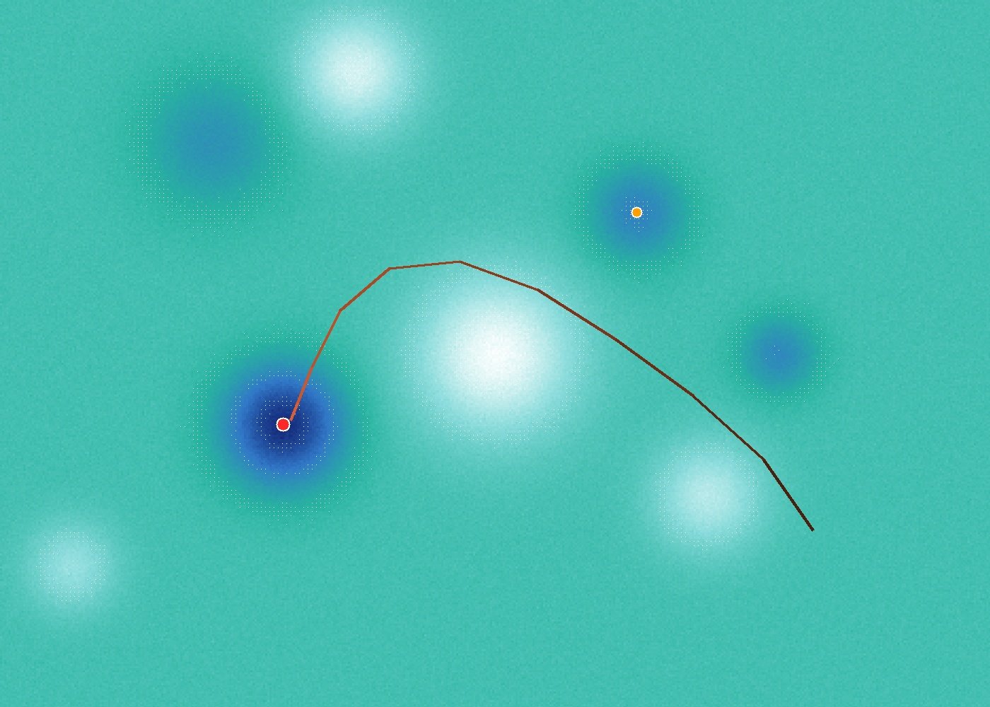
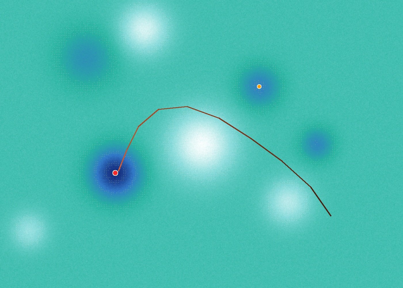
A 2D view of a loss landscape, with a gradient-descent trajectory toward a lower-loss minimum.
Loss is the score that training tries to lower
Language models learn by predicting what comes next. Give one a sequence of words and ask for the next token. The difference between its prediction and the token that actually appears is the signal that changes the model. That signal is called loss.
For language models, the usual measure is cross-entropy loss. At each step, the model assigns probabilities to possible next tokens. Cross-entropy compares those probabilities with the token that actually appeared. A confident, correct prediction produces little loss. A tiny probability on the correct token produces a sharp penalty.
Put more formally, loss is the negative log of the probability assigned to the correct token. The formula sounds like it escaped from a calculus lecture, but its job is simple: reward good predictions and punish bad ones in proportion to their confidence.
Scaling laws describe the relationship researchers plot between the number of parameters, dataset size, or compute, and the loss a model achieves.
Perplexity is loss raised as an exponent. It roughly describes how many equally likely choices the model seemed to be weighing at each step. On standard text benchmarks, a loss above 4 suggests a poorly trained or tiny model; 3 to 4 is mediocre; 2 to 3 is decent; and frontier models often sit around 1.5 or lower.
Training loss is calculated token by token and averaged across a batch. It is then backpropagated to update the model’s weights. Researchers also track loss on a held-out validation set, data the model did not train on, to see whether it is generalizing rather than memorizing. That validation loss is what appears on scaling-law curves.
Gradients tell the model where to move
A model needs a direction if it is going to reduce loss. That direction is the gradient.
The gradient is the derivative of loss with respect to each parameter. It describes whether a tiny change to a given weight raises or lowers loss, and by how much. In a model with billions of parameters, it is a vector with billions of numbers. Backpropagation calculates it by working backward through the network, layer by layer, using the chain rule to measure each parameter’s contribution to the final loss.
A loss landscape has hills and valleys, but one dimension for every parameter, which can mean billions of dimensions. At any point on that landscape, the gradient points in the direction of steepest increase. Gradient descent reduces loss by moving in the opposite direction, step by step down the loss surface.
The learning rate sets the size of each step. Set it too low and training crawls. Set it too high and the optimizer shoots past the valley it was trying to reach. A training schedule usually starts with small warmup steps, uses larger steps through the middle of training, then makes smaller adjustments near a good minimum.
At that point the model has settled into a stable set of weights. Continuing beyond convergence can lead to overfitting, when training loss keeps falling while validation loss rises.
Parameters and layers do different jobs
A parameter is one number stored inside a model. Every matrix weight and bias term counts. A 1,000-by-1,000 matrix contains one million parameters. Put dozens of layers together, each with matrices for attention and feed-forward operations, and the count reaches billions or trillions.
A layer is not the same thing as a matrix. It is a processing step that uses matrices as its main tool. Data enters as a vector; the layer multiplies it by a weight matrix, adds a bias vector, then applies a nonlinear activation function such as ReLU or GELU. Without that nonlinearity, many stacked layers would collapse mathematically into one large layer.
The layers progressively turn token data into representations useful for prediction. Early layers capture syntax and local word relationships. Later layers encode meaning, long-range context, and links between ideas far apart in the text.
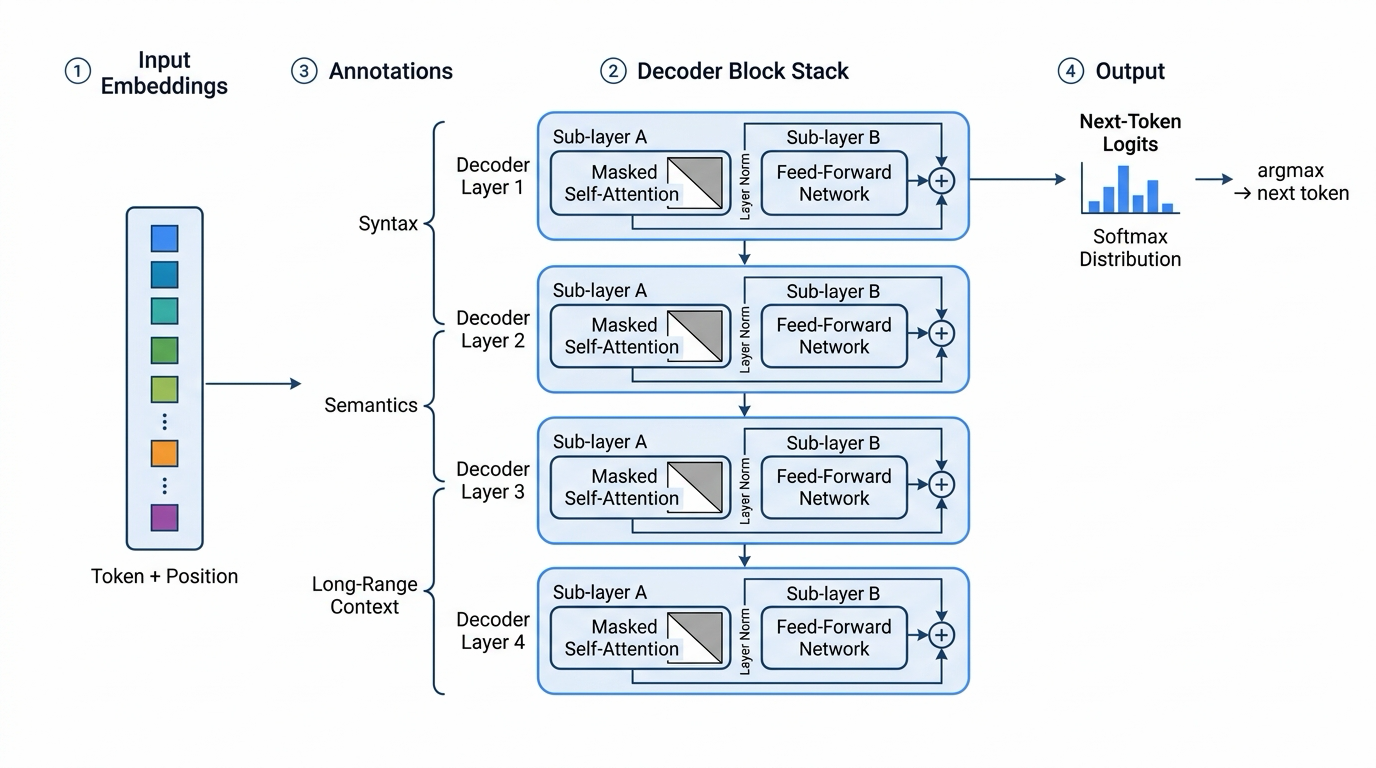
Layers refine raw token data into representations that help predict the next token.
Scaling laws make training less of a gamble
Model size and loss follow a power law. Plot loss against parameter count on a log-log scale and the result is a straight line. That lets researchers estimate a model’s quality before it is fully trained, which is a useful thing to know before somebody burns through a serious compute budget. Kaplan et al., “Scaling Laws for Neural Language Models” (OpenAI, 2020)
OpenAI’s 2020 work, led by Jared Kaplan, established the early scaling-law picture. DeepMind’s 2022 Chinchilla paper revised a key assumption. Kaplan’s team argued for scaling parameters faster than data; Chinchilla found that approach suboptimal. For a fixed compute budget, its result was to scale parameters and training tokens roughly equally, at about 20 tokens per parameter. Hoffmann et al., “Training Compute-Optimal Large Language Models” (DeepMind, 2022)
Long context has a weak spot in the middle
Very deep networks have a known problem: vanishing gradients. As a gradient moves backward through many layers, its signal can weaken enough that early layers barely update. Residual connections help by adding a layer’s input directly to its output, giving gradients a more direct route. Modern transformers use them.
Long context creates a related but separate problem. Information at the beginning of a long document must survive repeated mixing across subsequent layers and attention steps. Along the way, its signal can get diluted.
Researchers call one version of this the “lost in the middle” effect. Models are noticeably worse at retrieving information from the middle of a long context than from the beginning or the end. Liu et al., “Lost in the Middle: How Language Models Use Long Contexts” (2023)
Two mechanisms compound the problem. Attention has positional biases: models tend to weight early tokens and tokens near the current prediction point more heavily. Middle tokens receive less attention at each layer, and that disadvantage compounds with depth.
Training data adds another bias. In typical documents, important information often sits at the beginning or end. Models learn to favor those positions because the shortcut worked in training, then carry it over when the important detail is buried in the middle.
Rotary position embeddings (RoPE) encode position by rotating token vectors. They represent nearby, well-anchored positions more cleanly than arbitrary positions deep in a long sequence. The geometry is less precise in the middle.
Bigger context windows do not solve retrieval by themselves
Subquadratic is working on the compute cost of long context. Its first model, SubQ 1M-Preview, uses what the company calls Subquadratic Sparse Attention, an architecture where compute grows linearly with context length rather than roughly quadratically as in standard attention. The company reports a context window of up to 12 million tokens, plans for a 50-million-token model, and $29M in funding. Subquadratic company announcements (2025)
Those claims address cost and scale. The “lost in the middle” effect asks a different question: whether a model can use the right information once that information is in the window. A model may process 12 million tokens affordably and still miss the one detail that matters. Independent researchers have asked for verification of Subquadratic’s efficiency claims, so those numbers remain unverified for now.
Neither problem is a permanent ceiling. Researchers are iterating on positional encoding, and they are building training examples that place the answer in the middle of the context so models have to unlearn the positional shortcut. Bigger windows may be impressive. Better use of what is inside them is the harder test.
Sources
Kaplan et al., “Scaling Laws for Neural Language Models,” OpenAI, 2020; Hoffmann et al., “Training Compute-Optimal Large Language Models” (Chinchilla), DeepMind, 2022; Liu et al., “Lost in the Middle: How Language Models Use Long Contexts,” 2023; Subquadratic company announcements, 2025.